
Linear Optimization
Many quantitative decision tasks in economy and industry lead naturally to optimization problems. A broad category of practically tractable problems are linear optimization problems where the goal function and the constraints depend linearly on the decision variables. Let us illustrate the linear optimization (also called linear programming) on an example from the mining industry.
Optimization Model
A mining company extracts rock or minerals from an open pit (quarry), mixes them to achieve the required quality and sells the blend on the market. The company wants obviously achieve a maximum profit under the constraints given by the quarry composition, the mix, production costs and capacity. The situation can be modeled mathematically as follows.
Discretization
The quarry is divided into more or less homogeneous blocks:
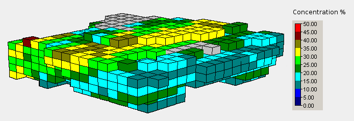
Block model of a quarry
Data
The mineral concentration, the weight, the production cost and other properties of the blocks are measured or estimated:
| Block | Tonnage | Profit c/ton | R % | S % |
|---|---|---|---|---|
| B1 | 20 | 6 | 15 | .. |
| B2 | 10 | 2 | 35 | .. |
| B3 | .. | .. | .. | .. |
Quarry data
Maximum function
The goal is to maximize the profit
by taking
x1 tons from the block B1,
x2 tons from the block B2,
...
and satisfying all constraints that follow below.
Requirements on the blend
The concentration of the chemicals in the blend must lay between specified limits:
| Chemical | Min % | Max % |
|---|---|---|
| R | 20 | 25 |
| S | .. | .. |
| .. | .. | .. |
Requirements on the chemical mix
This means for the chemical R:
x1 + x2 + ...
This is reformulated as two inequalities:
Corresponding inequalities are added for further chemicals.
Natural constraints on the tonnage
The taken tonnages must satisfy the obvious constraints:
Limited production capacity
The company has only a limited production capacity Tmax:
Two-dimensional case
We will now solve the problem in the simplified case of 2 blocks only. We assume that the maximum production capacity is Tmax = 25 tons. The task is then: Find the variables x1, x2 such that the profit
is maximal and the constraints:
are satisfied. This kind of problems are called linear optimization problems because the function to be optimized and all restrictions are linear functions in the variables x. Treatment of these problems and the corresponding solution methods is also called - for historical reasons - linear programming.
Graphical solution
In the case of 2 variables the problem can be solved graphically in the (x1, x2)-plane.
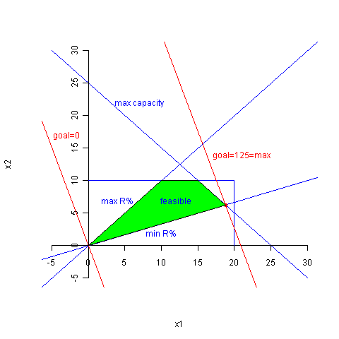
Graphical solution (Picture creation)
The inequalities correspond to half-planes bounded by the constraint equations (inequality replaced by equality). The intersection of these half-planes is a convex polygon called the "feasible region". The points of the feasible region satisfy all constraints. The goal corresponds to a family of parallel lines
parametrized by the value of m. When this line is moved to the right, the value m of the goal is increased and it achieves the maximum 125 at the right most corner (18.75, 6.25) of the feasible region. So, the optimal solution is
The graphical solution method provides an excellent insight into the structure of linear optimization problems. Even if we cannot use it directly in higher dimensions, we can imagine how it would work. Constraints correspond to half-spaces bounded by hyperplanes. The feasible region, which is the intersection of half-spaces, is a convex polyhedron. The goal is a hyperplane that must be moved to that vertex of the polyhedron where its value is maximal.
Solution with Microsoft Excel
Microsoft Excel provides the add-on "Solver" that allows to solve optimization problems numerically. The application of Excel Solver (PDF) to our two-dimensional example is easy. However, the Solver becomes impractical and error-prone for real-world large scale problems.
Simplex Algorithm
Simplex Algorithm (PDF)is the method of choice for linear optimization of real-world large scale problems. This method was devised by G. B. Dantzig in 1947. My implementation of the Simplex Algorithm in C++ can handle thousands of variables and constraints, is numerically stable and computes the solution very efficiently.