
Modelling Disease Spread
Spread of infectious diseases can be investigated by means of mathematical models.
The I-Model
The I-model is the simplest exponential model for disease spread. It focuses only on the number I of infected people. All infected people will also recover.
Let us assume that at day 0 one person - the so called patient zero - is ill. The patient 0 infects 2 person during 1 day and becomes healthy at the same time. So on day 1 there are 2 persons ill. Each of them infects ahain 2 persons during one day and recovers himself. So, on day 2 there are 4 persons ill. If this procedure continues the disease spreads as depicted in the figures below:
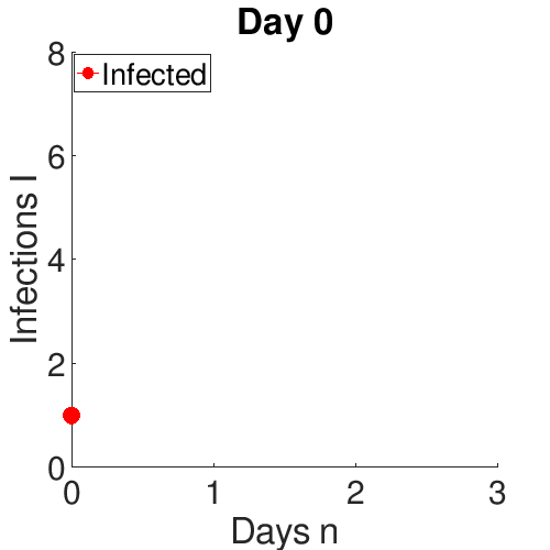
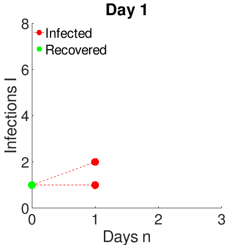
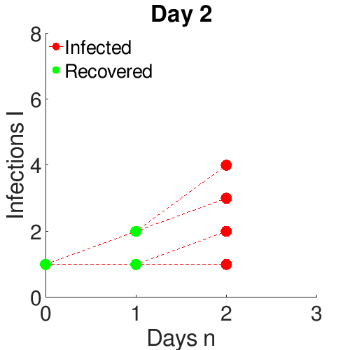
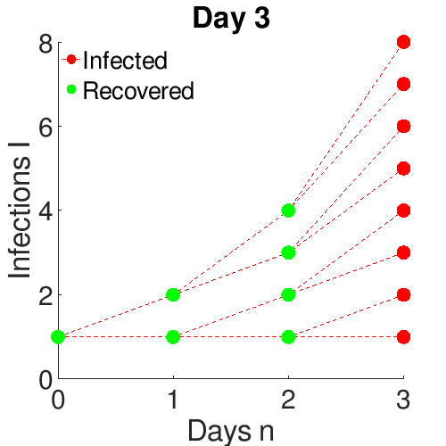
We denote by $I_n$ the cumulative number of people that have been infected from the first day until the day $n$. We observe that that this number is: $$\begin{align} I_0 & = 1 \\ I_1 & = 2 \cdot 1 = 2 \\ I_2 & = 2 \cdot 2 = 4 \\ I_3 & = 2 \cdot 4 = 8 \end{align}$$ In general we have: $$\begin{align} I_0 & = 1 \tag {1a} \\ I_n & = 2 \cdot I_{n-1} \tag {1b} \\ I_n & = 2^n \tag {1c} \end{align}$$
The cumulative number of recovered people $R_n$ on day $n$ is: $$\begin{align} R_0 & = 0 \\ R_n & = I_0 + I_1 + ... + I_{n-1} = 1 + 2 + 2^2 + ... + 2^{n-1} \\ R_n & = 2^{n} - 1 , n \gt 0 \tag {2a} \\ R_n & = I_n - 1 , n \gt 0 \tag {2b} \end{align}$$
The number of infected people grows exponentially:
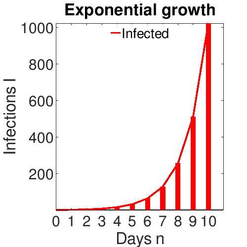
The grows at the beginning is slow and the spread of the disease is underestimated. The spread becomes monstreous fast:
- after 5 days 32 people are infected - a small group
- after 10 days 1 thousand (1,032) people are infected - a small town
- after 20 days 1 million people (1,048,576) are infected - a city
- after 33 days 8 billion people (8,589,934,592) are infected - the whole world.
Reproduction number $\pmb R_0$
We will generalize the I-model as folows. Suppose that there are $I(0)$ people infected at time 0. Each one infects $\pmb R_0$ people during $T$ days. The number of infected people after $k T$ days is hence:
$$ I(kT) = I(0) {\pmb R_0} ^ k \tag {3} $$We get the number of infected people for an arbitrary time $t$ by setting $t = k T$:
$$ I(t) = I(0) {\pmb R_0} ^ {t / T} \tag {4} $$The number $\pmb R_0$ is called the reproduction number and plays a crucial role for the disease spread. We see from Eq. (4) that: $$\begin{align} \pmb R_0 \gt 1 & \Rightarrow \text{exponential growth} \tag {5a} \\ \pmb R_0 = 1 & \Rightarrow \text{constant} \tag {5b} \\ \pmb R_0 \lt 1 & \Rightarrow \text{exponential decrease} \tag {5c} \end{align}$$
One person infects $$ \pmb R_1 := {\pmb R_0} ^ {1 / T} \tag {6} $$ persons in 1 day. Eq. (4) can be witten as $$ I(t) = I(0) {\pmb R_1} ^ t \tag {7} $$ Since $$ \pmb R_0 \lesseqgtr 1 \Longleftrightarrow \pmb R_1 \lesseqgtr 1 \tag {8} $$ we see that the period $T$ is irrelevant for the distinction whether the contagion spreads or decreases.
The following table shows the reproduction number for well-known infectious deseases:
| Desease | $\pmb R_0$ |
|---|---|
| Measles | 12 - 18 |
| Mumps | 10 - 12 |
| Polio | 5 - 7 |
| HIV / AIDS | 2 - 5 |
| SARS | 0.2 - 1.1 |
| SARS-CoV-2 / COVID-19 | 2 - 6 |
| Common cold | 2 - 3 |
| Diphtheria | 1.7 - 4.3 |
| Ebola | 1.5 - 1.9 |
| Influenza | 1.4 - 1.6 |
| MERS | 0.3 - 0.8 |
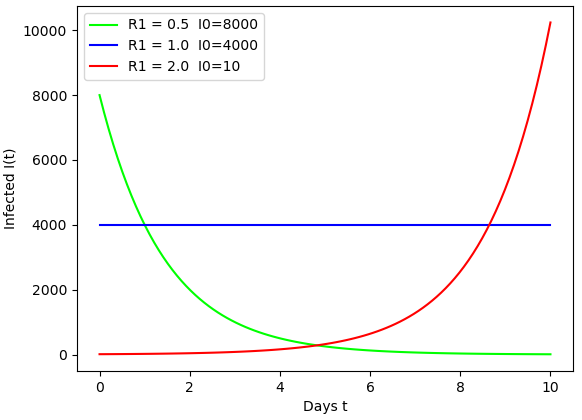
The following figure shows the desease spread for various values of $\pmb R_1$:
The cumulative number of Covid-19 infections for Italy (1-March-2020 - 30-June-2020)
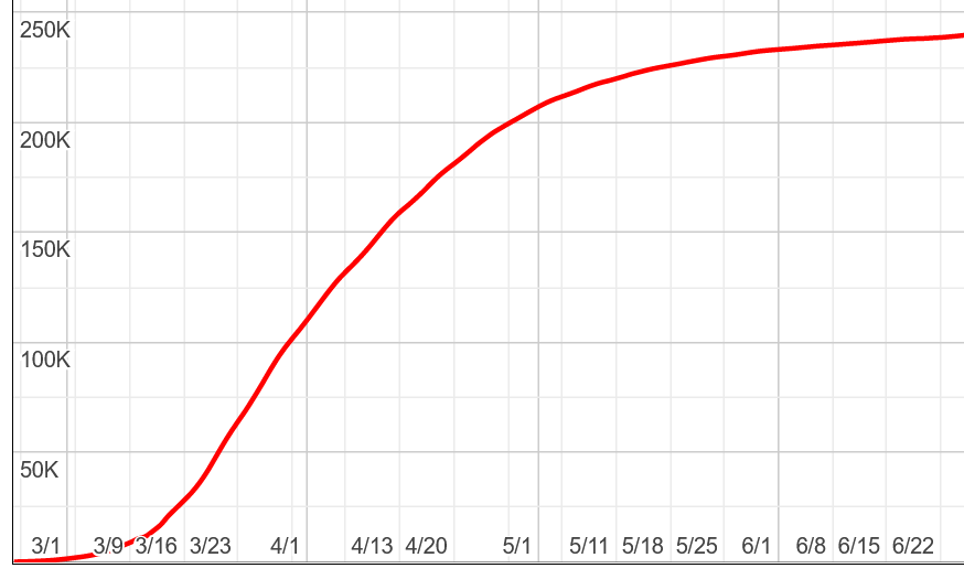
grows exponentially only at the beginning of the epidemy but flattens during the time. The cause is mainly due to limiting measures ("lockdown") that reduce the number of contacts. But there is also a fundamental reason for slowing down: the number of all people is finite and hence the number of people who can get infected in the future decreases. During the time the infected people do not have many opportunities to infect further people.
The SI-Model
A more realistic way of modelling the spread of disease is using the SI model. The main characteristics of this model is that it takes into account the finite number of people. The whole population of $N$ people is divided into 2 categories called compartments: people who are susceptible $S$ and people who are infectious $I$.
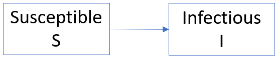
Infected people infect the susceptible people who become infected and remain infected. So, there is a "flow" of people from the S-compartment to the I-compartment. However, the total number of people remains constant at all times $t$: $$ S(t) + I(t) = N \tag {9} $$ During the time period $\Delta t$ one infected person contacts $c \Delta t$ other people where $c$ is number of people contacted in time unit (a day). Since the proportion of susceptible people is $S / N$ there are $c (S / N) \Delta t$ susceptible people among these contacts. If the probability of "disease transmission" is $p_t$ then one infected person infects $$ p_t c (S / N) \Delta t = \beta (S / N) \Delta t \tag {10} $$ people, where we introduced the constant $$ \beta = p_t c = \text{transmission probability * contact rate} \tag {11} $$ All $I$ infected persons infect $$ \Delta I = p_t c I \frac{S}{N} \Delta t = \beta I \frac{S}{N} \Delta t \tag {12a} $$ people. The number of susceptible people decreases correspondingly: $$ \Delta S = - \beta I \frac{S}{N} \Delta t \tag {12b} $$
With the introduction of differential and proportional quantities:
- $\Delta S / \Delta t \approx dS /dt$
- $\Delta I / \Delta t \approx dI /dt$
- $s = S / N$ the proportion of the population who are susceptible
- $i = I / N$ the proportion of the population who are infected
we get two differential equations for the development of the disease: $$\begin{align} \frac{si}{dt} & = - \beta i s \tag {13a} \\ \frac{di}{dt} & = \beta i s \tag {13b} \end{align}$$
The equations can be solved in a closed form. We write Eq. (13b) as $$ \frac{di}{dt} = \beta i (1 - i) \tag {14} $$ separate the variables $$ \frac{di}{i (1 - i) } = \beta dt \tag {15} $$ and integrate $$ \int_{i_0}^{i} \frac{di}{i (1 - i) } = \int_{0}^{t} \beta dt \tag {16} $$ The integral on the left side can be evaluated by considering $$ \frac{1}{i (1 - i)} = \frac{1}{i} + \frac{1}{1 - i} \tag {17} $$ We get $$\begin{align} \ln i - \ln (1 - i) & = \beta t + const \\ \ln \frac{i}{1-i} & = \beta t + const \\ \frac{i}{1-i} & = e^ {\beta t + const} = A e^ {\beta t} \tag {18} \end{align}$$ We obtain the value of the constant $A$ by setting $i(0) = i_0$: $$ A = \frac{i_0}{1 - i_0} \tag {19} $$ Finally we solve Eq. 18 for $i$ and get $$ i(t) = \frac{A e^{\beta t} } {1 + A e^{\beta t}} \tag {20} $$ Eq. (20) is a type of "logistic equations" that are used for modelling of population growth restrained to limiting resources. In our case the "population" are the infected people who increase and the "limited resource" are the sustainable people who decrease.
The folowing figure shows an example of the function (20). Notice that $$ s(t) = 1 - i(t) \tag {21} $$
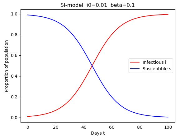
We observe the typical S-shape of the "sigmoid" curve. The curve matches much better the real spread of Covid-19.
The SIR-Model
A still better model is the SIR model that was introduced already in 1927 by Kermack and McKendrick. The whole population of $N$ people is divided into 3 compartments: people who are susceptible $S$, people who are infectious $I$ and people who have recovered $R$:
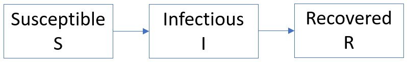
A more general interpretation of the compartment $R$ is "Remaining" or "Removed" people: those people who are neither susceptible nor infected. These are people who have recovered or died or are immune against the disease. The "Infectious" people are also call "Infectives" or "Infected". We assume that "infected" people are "infectious".
We suppose that if there are $I(t)$ infected people then the fraction of them $$ \Delta I = \gamma I \Delta t \tag {22} $$ recover in time $\Delta t$. Hence we get the following differential equations for the relative quantities: $$\begin{align} \frac{ds}{dt} & = - \beta i s \tag {23a} \\ \frac{di}{dt} & = \beta i s - \gamma i \tag {23b} \\ \frac{dr}{dt} & = \gamma i \tag {23c} \end{align}$$
These equations cannot be solved analytically but only numerically. Two solutions for different parameters are shown below:
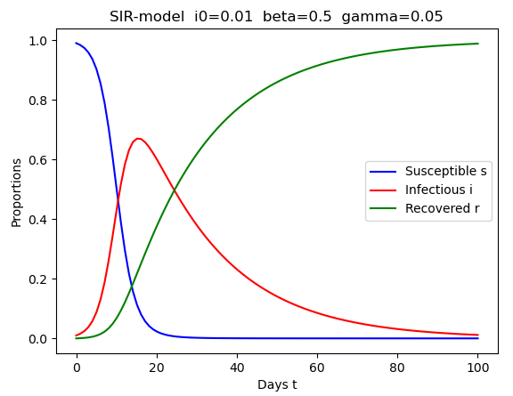
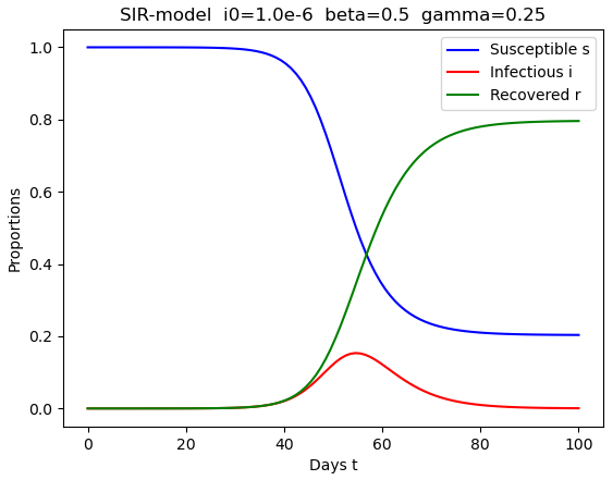
Python integration of SIR differential equations.
Reproduction number in the SIR-Model
The epidemiological definition of the reproduction number $\pmb R$ is the average number of secondary cases produced by one infected individual introduced into a population of susceptible individuals. We saw above that one infected person infects $$ \beta \frac{S}{N} \Delta t = \beta s \Delta t \tag {24} $$ people in time $\Delta t$. If $\Delta t$ equals the time when the person is infectious then Eq. (24) defines $\pmb R$. How long is a person infectious? When all people $I(t)$ infected at time $t$ recover after time $T$ then $T$ is the duration of infection. Using Eq. (22) we obtain $T$: $$\begin{align} \Delta I & = I \\ \gamma I(t) T & = I(t) \\ T & = \frac{1}{\gamma} \tag {25} \end{align}$$ Substituing Eq. (25) into Eq. (24) we get $$ \pmb R(t) = \frac{\beta}{\gamma} s(t) = \frac{s(t)}{\rho} \tag {26} $$ where we introduced the constant $$ \rho = \frac{\gamma}{\beta} \tag {27} $$ $\pmb R(t)$ is called the effective reproduction number. It decreases during the epidemic because the number of susceptible people dicreases. The basic reproduction number is the effective reproduction number at time 0: $$ \pmb R_0 = \frac{s_0}{\rho} \tag {28} $$ and determines whether the disease will spread or disappear. At the beginning of the epidemic we have approximatively: $$ s(t) \approx s_0 \tag {29} $$ such that Eq. (23b) becomes: $$ \frac{di}{dt} \approx \beta i s_0 - \gamma i = \gamma (\pmb R_0 - 1) i \quad \text{(for t small)} \tag {30} $$ The solution of this equation is $$ i(t) \approx i_0 e ^ {\gamma (\pmb R_0 - 1) t} \quad \text{(for t small)} \tag {31} $$ If $\pmb R_0 \gt 1$ the disease will spread, if $\pmb R_0 \lt 1$ the disease will die out.
Progression of the disease in the SIR-model
In the last section we saw how the disease behaves at the beginning of the outbreak. We will now investigate the furher progression of the disease. It is sufficient to consider only the equations (23a) and (23b), because $r(t) = 1 - s(t) - i(t)$.
Since $ds/dt \ne 0$ we can divide (23b) by (23a) to get a differential equation for $i(s)$: $$ \frac{di(s)}{ds} = \frac{\rho}{s} - 1 \tag {32} $$ The integration is easy and yields: $$ i(s) = \rho \; ln s - s + c_0 \tag {33} $$ where we introduced the constant $c_0$: $$ c_0 = i_0 + s_0 - \rho \; ln s_0 \tag {34} $$ The equation (33) is defined in the triangular region of the phase space $s/i$: $$ 0 \le s, i(s) \le 1 \text{ and } s + i(s) \le 1 \tag {35} $$ We can always assume that $$ i_0 + s_0 = 1 \tag {36} $$ which corresponds to $r_0 = 0$. If there were recovered poeple at the beginning we could immediately exclude them from the population. The following figure shows $i(s)$ for various initial values $s_0$.
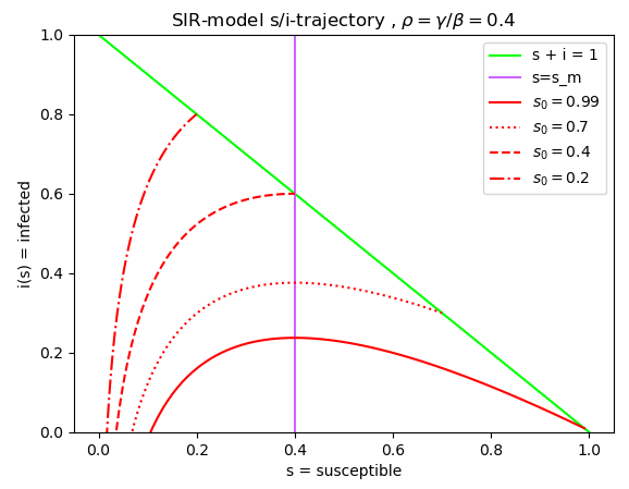
The curves $i(s)$ in the phase plane $s/i$, called 'trajectories', correspond to the curves $(t, s(t)), (t, i(t))$ in the $t/(s, i)$ space. The curves start with different initial values $s_0, i_0 = 1 - s_0$ but with the same parameter $\gamma$. Since $ds/dt \lt 0$, $s(t)$ decreases with increasing time, so the trajectories $i(s)$ start at the right end and progress to the left. The maximum of $i(s)$ is achieved at $s_{max}$ where Eq. (33) is zero but only if $i(\rho) \le 1 - \rho$: $$ s_{max} = \begin{cases} \rho & \text{if } \; i(\rho) \le 1 - \rho \tag {37} \\ s_0 & \text{if } \; i(\rho) \ge 1 - \rho \end{cases} $$ After $i(s)$ achieved its maximum it decreases for $s \to 0$ (i.e. for $t \to \infty$). Finally, $i(s)$ becomes 0 at $s = s_\infty$ which is the solution of the equation: $$ i(s_\infty) = \rho \; ln s_\infty - s_\infty + c_0 = 0 \tag {38} $$ This equation has always a positive solution $s_\infty$ because $i(s_{max}) \gt 0$ and $i(s=0) = - \infty \lt 0$, such that $i(s)$ crosses the horizontal axis. Eq. (38) can be solved in closed form by refering to the Lambert $W$ function. First, the equation is rewritten as $$ s = e^{- c_0 / \rho} e^{s / \rho} $$ The solution is then $$ s_\infty = -\rho \; W \left( - \frac{1}{\rho} \; e^{-c_0 / \rho } \right) \tag {39} $$ As $i(s)$ approches $0$, $ds/dt$ approaches 0 as well. So there is no final time $t$ such that $s(t) = s_\infty$ but only a limit. Summarizing, we obtain the following limiting values: $$\begin{align} \lim_{t \to \infty} s(t) & = s_{\infty} > 0 \tag {40a} \\ \lim_{t \to \infty} i(t) & = 0 \tag {40b} \end{align}$$ These limiting equations are also called "final size relation". It is worth to stress that any epidemic dies finally out according to the SIR-model even if it can take a long time. At the end there are no infected people even if susceptible people may remain. This behaviour is valid for any initial conditions and any parameters.
Total number of infected people in the SIR-model
How many people get infected during the epidemy? These are the people who passed through the I-compartment to the R-compartment, so people who recovered or died. The proportion of these people with respect to the whole population is $$ i_{total} = \int_{0}^{\infty} i(t) dt = r_\infty = 1 - s_\infty \tag {41} $$ because $i_\infty = 0$.
Herd immunity in the SIR-model
A population exhibits herd immunity if the disease does not spread. Herd immununity can be achieved by vaccination. Let us assume that $p_v$ percent of the population are vaccinated and immune at the beginning of the epidemic. This means that the number of susceptible people at time $t = 0$ is reduced to $s'_0 = (1 - p_v) s_0$. We request that the reproduction number in this new population is less than 1 to prevent spread of the disease: $$ \pmb R'_0 = \frac{s'_0}{\rho} = \frac{s_0 (1 - p_v)}{\rho} = \pmb R_0 (1 - p_v) \lt 1 \tag {42} $$ Solving this inequality for $p_v$ we get $$ p_v > 1 - \frac{1}{\pmb R_0} \tag {43} $$ In case of Covid-19 $\pmb R_0$ is approximatively 3, resp. 4, such that more that 66%, resp 75% of the population need to be vaccinated to prevent the spread.
Advanced models
The SIR-model can be further extended and refined by introducing further compartments. Besides these deterministic models there are also stochastic and other models that can be found in the literature and online.
References
- Spread of Disease by Julia Collins and Nadia Abdelal
- Basic reproduction number (Wikipedia)
- Compartmental models (Wikipedia)
- Asymptotical behavior of the SIR epidemic model (StackExchange / Mathematics)
- Lambert W function (Wikipedia)